How To Draw To Different Graphs In A Single Viewer In Graphstream

Welcome! If yous've always wanted to larn and empathise Dijkstra's algorithm, and so this article is for you. You lot will see how it works behind the scenes with a step-past-stride graphical explanation.

You will acquire:

• Basic Graph Concepts (a quick review).
• What Dijkstra'due south Algorithm is used for.
• How it works backside the scenes with a step-by-step example.

Let's begin. ✨

🔹 Introduction to Graphs

Let's start with a brief introduction to graphs.

Basic Concepts

Graphs are data structures used to represent "connections" betwixt pairs of elements.

• These elements are called nodes. They represent real-life objects, persons, or entities.
• The connections between nodes are called edges.

This is a graphical representation of a graph:

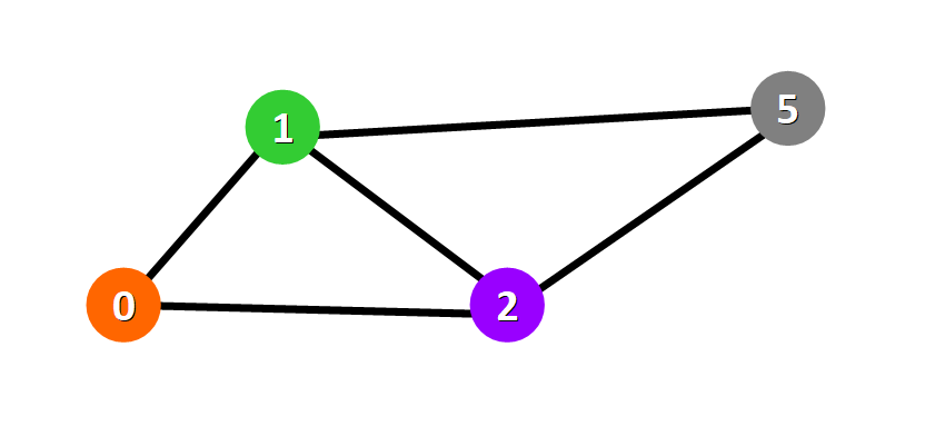
Nodes are represented with colored circles and edges are represented with lines that connect these circles.

💡 Tip: Two nodes are continued if there is an edge between them.

Applications

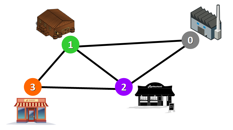
Graphs are directly applicative to real-earth scenarios. For example, we could use graphs to model a transportation network where nodes would correspond facilities that send or receive products and edges would represent roads or paths that connect them (see below).

Network represented with a graph

Types of Graphs

Graphs tin be:

• Undirected: if for every pair of connected nodes, you tin go from i node to the other in both directions.
• Directed: if for every pair of connected nodes, you lot can only go from ane node to another in a specific direction. We use arrows instead of elementary lines to represent directed edges.

💡 Tip: in this article, we will work with undirected graphs.

Weighted Graphs

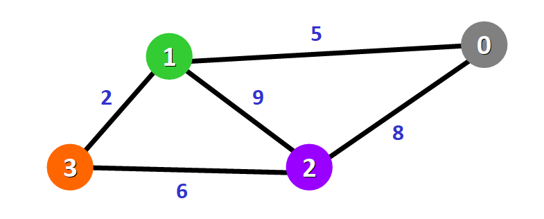
A weight graph is a graph whose edges have a "weight" or "cost". The weight of an edge can stand for altitude, fourth dimension, or anything that models the "connection" between the pair of nodes it connects.

For example, in the weighted graph below you can come across a blue number adjacent to each edge. This number is used to represent the weight of the respective edge.

💡 Tip: These weights are essential for Dijkstra's Algorithm. You lot will see why in but a moment.

🔸 Introduction to Dijkstra'due south Algorithm

At present that yous know the basic concepts of graphs, let's beginning diving into this amazing algorithm.

• Purpose and Use Cases
• History
• Basics of the Algorithm
• Requirements

Purpose and Employ Cases

With Dijkstra's Algorithm, you can find the shortest path between nodes in a graph. Specially, y'all can find the shortest path from a node (called the "source node") to all other nodes in the graph, producing a shortest-path tree.

This algorithm is used in GPS devices to detect the shortest path between the current location and the destination. It has broad applications in manufacture, especially in domains that require modeling networks.

History

This algorithm was created and published by Dr. Edsger W. Dijkstra, a bright Dutch calculator scientist and software engineer.

In 1959, he published a three-folio article titled "A note on two problems in connexion with graphs" where he explained his new algorithm.

Dr. Edsger Dijkstra at ETH Zurich in 1994 (image past Andreas F. Borchert)

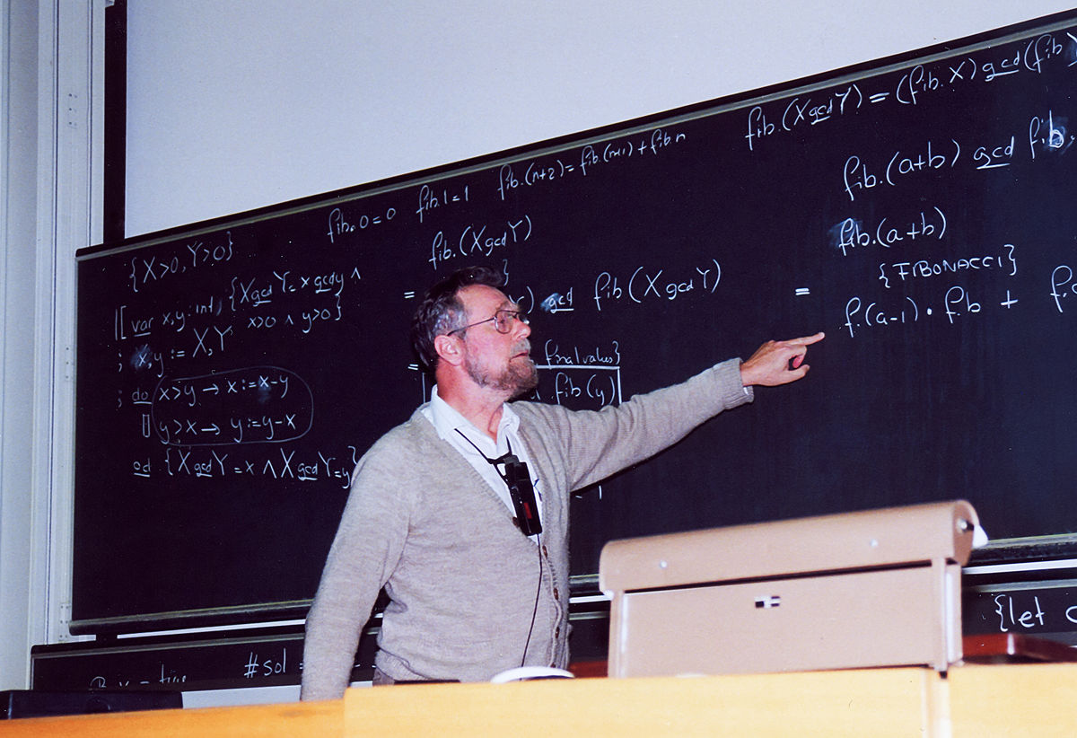
During an interview in 2001, Dr. Dijkstra revealed how and why he designed the algorithm:

What's the shortest way to travel from Rotterdam to Groningen? Information technology is the algorithm for the shortest path, which I designed in about 20 minutes. One morn I was shopping in Amsterdam with my young fiancée, and tired, nosotros sabbatum down on the café terrace to drink a cup of coffee and I was just thinking about whether I could do this, and I then designed the algorithm for the shortest path. Equally I said, information technology was a 20-infinitesimal invention. In fact, information technology was published in 1959, three years later. The publication is yet quite nice. One of the reasons that it is so nice was that I designed it without pencil and newspaper. Without pencil and paper you lot are almost forced to avoid all avoidable complexities. Somewhen that algorithm became, to my great amazement, i of the cornerstones of my fame. — Every bit quoted in the article Edsger W. Dijkstra from An interview with Edsger W. Dijkstra.

⭐ Unbelievable, right? In just 20 minutes, Dr. Dijkstra designed one of the well-nigh famous algorithms in the history of Computer Scientific discipline.

Nuts of Dijkstra's Algorithm

• Dijkstra'due south Algorithm basically starts at the node that you cull (the source node) and it analyzes the graph to observe the shortest path between that node and all the other nodes in the graph.
• The algorithm keeps track of the currently known shortest distance from each node to the source node and it updates these values if it finds a shorter path.
• One time the algorithm has institute the shortest path between the source node and another node, that node is marked every bit "visited" and added to the path.
• The process continues until all the nodes in the graph have been added to the path. This way, we have a path that connects the source node to all other nodes following the shortest path possible to attain each node.

Requirements

Dijkstra'south Algorithm can only work with graphs that take positive weights. This is considering, during the procedure, the weights of the edges take to be added to find the shortest path.

If there is a negative weight in the graph, then the algorithm will not work properly. One time a node has been marked as "visited", the current path to that node is marked as the shortest path to reach that node. And negative weights tin alter this if the full weight can be decremented after this step has occurred.

🔹 Case of Dijkstra'due south Algorithm

Now that you know more about this algorithm, let's come across how it works behind the scenes with a a pace-by-pace example.

We take this graph:

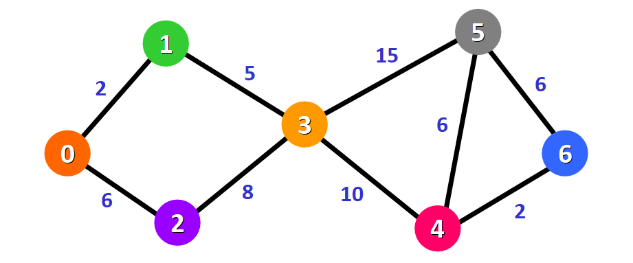
The algorithm volition generate the shortest path from node 0 to all the other nodes in the graph.

💡 Tip: For this graph, we will assume that the weight of the edges represents the distance between two nodes.

We volition have the shortest path from node 0 to node 1, from node 0 to node two, from node 0 to node 3, then on for every node in the graph.

Initially, we have this list of distances (please see the list below):

• The distance from the source node to itself is 0. For this case, the source node volition be node 0 but it can be any node that you choose.
• The altitude from the source node to all other nodes has not been determined yet, so we use the infinity symbol to correspond this initially.

We besides accept this list (see below) to keep track of the nodes that have not been visited however (nodes that have not been included in the path):

💡 Tip: Remember that the algorithm is completed once all nodes accept been added to the path.

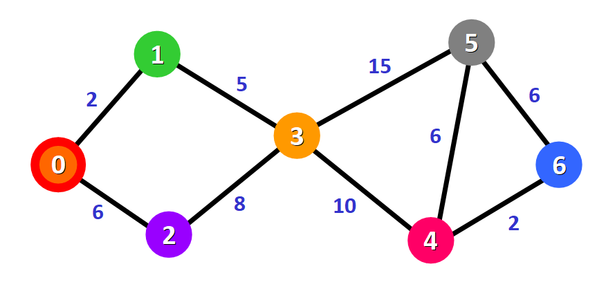
Since we are choosing to start at node 0, we can marker this node as visited. Equivalently, we cross it off from the list of unvisited nodes and add a scarlet border to the corresponding node in diagram:

At present nosotros need to beginning checking the distance from node 0 to its adjacent nodes. Every bit you lot tin can see, these are nodes i and 2 (see the red edges):

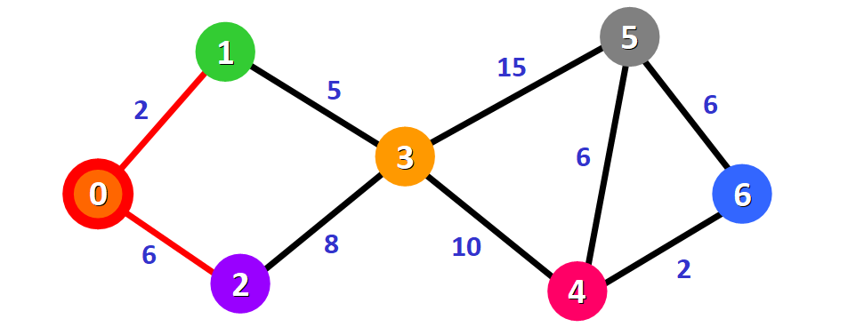
💡 Tip: This doesn't mean that we are immediately adding the two next nodes to the shortest path. Earlier adding a node to this path, nosotros need to check if we accept institute the shortest path to reach it. We are simply making an initial examination process to see the options available.

We need to update the distances from node 0 to node one and node two with the weights of the edges that connect them to node 0 (the source node). These weights are ii and vi, respectively:

After updating the distances of the adjacent nodes, nosotros demand to:

• Select the node that is closest to the source node based on the current known distances.
• Mark it every bit visited.
• Add it to the path.

If we check the listing of distances, nosotros tin see that node 1 has the shortest distance to the source node (a distance of two), and then we add information technology to the path.

In the diagram, we can represent this with a red border:

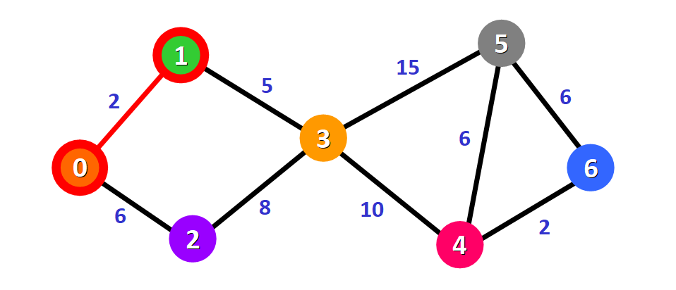
We mark it with a red square in the listing to represent that it has been "visited" and that we have found the shortest path to this node:

We cross information technology off from the list of unvisited nodes:

At present we need to analyze the new adjacent nodes to find the shortest path to reach them. Nosotros will only analyze the nodes that are side by side to the nodes that are already role of the shortest path (the path marked with red edges).

Node three and node ii are both adjacent to nodes that are already in the path considering they are directly continued to node one and node 0, respectively, every bit y'all can encounter below. These are the nodes that we will analyze in the next footstep.

Since we already have the altitude from the source node to node two written downwardly in our list, we don't demand to update the distance this time. Nosotros merely need to update the distance from the source node to the new adjacent node (node 3):

This altitude is 7. Let's come across why.

To find the distance from the source node to another node (in this example, node 3), we add the weights of all the edges that course the shortest path to accomplish that node:

• For node 3: the total distance is 7 considering we add together the weights of the edges that form the path 0 -> 1 -> 3 (2  for the border 0 -> i and v for the edge one -> iii).

Now that we have the distance to the adjacent nodes, we have to choose which node will exist added to the path. We must select the unvisited node with the shortest (currently known) distance to the source node.

From the list of distances, nosotros can immediately detect that this is node 2 with distance 6:

We add together information technology to the path graphically with a red border around the node and a red edge:

We too mark it as visited by calculation a small-scale red square in the list of distances and crossing information technology off from the list of unvisited nodes:

Now we need to repeat the process to find the shortest path from the source node to the new next node, which is node 3.

You can run across that we have 2 possible paths 0 -> 1 -> three or 0 -> 2 -> three. Let's encounter how we can decide which ane is the shortest path.

Node 3 already has a distance in the list that was recorded previously (7, see the list below). This altitude was the effect of a previous step, where we added the weights 5 and 2 of the two edges that we needed to cantankerous to follow the path 0 -> 1 -> 3.

Simply at present we have another culling. If nosotros choose to follow the path 0 -> 2 -> 3, we would need to follow ii edges 0 -> 2 and 2 -> iii with weights half dozen and viii, respectively, which represents a full altitude of xiv.

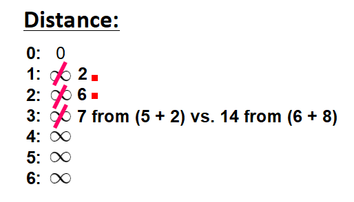
Clearly, the first (existing) distance is shorter (vii vs. 14), so we will choose to keep the original path 0 -> 1 -> 3. We but update the distance if the new path is shorter.

Therefore, we add this node to the path using the first alternative: 0 -> i -> three.

We marker this node as visited and cross information technology off from the list of unvisited nodes:

At present we repeat the process again.

Nosotros need to check the new adjacent nodes that we have non visited so far. This fourth dimension, these nodes are node four and node 5 since they are adjacent to node iii.

Nosotros update the distances of these nodes to the source node, always trying to discover a shorter path, if possible:

• For node iv: the distance is 17 from the path0 -> 1 -> 3 -> 4.
• For node 5: the altitude is 22 from the path 0 -> i -> iii -> 5.

💡 Tip: Notice that we tin only consider extending the shortest path (marked in cherry-red). Nosotros cannot consider paths that will take us through edges that have non been added to the shortest path (for instance, we cannot form a path that goes through the edge 2 -> 3).

Nosotros need to cull which unvisited node will exist marked as visited now. In this case, it'due south node 4 because it has the shortest distance in the list of distances. We add it graphically in the diagram:

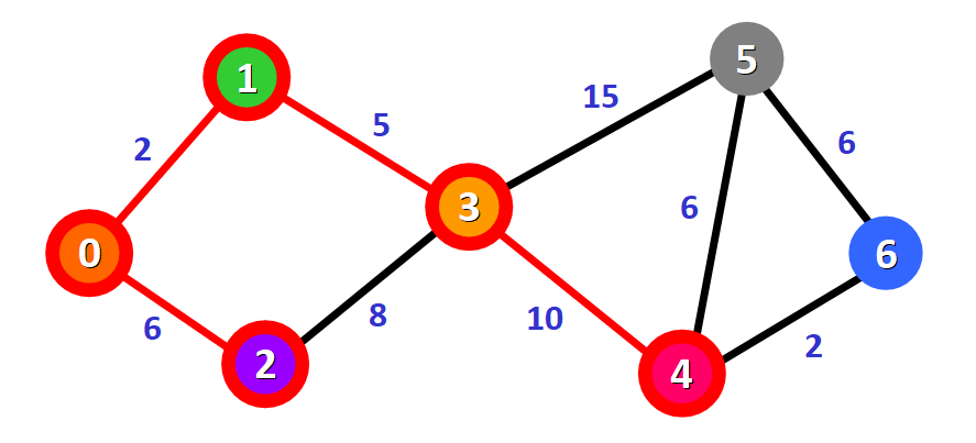
We too mark it as "visited" by adding a small cherry-red square in the listing:

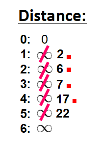
And we cross it off from the listing of unvisited nodes:

And nosotros repeat the procedure again. We bank check the adjacent nodes: node 5 and node 6. We need to clarify each possible path that we can follow to reach them from nodes that take already been marked as visited and added to the path.

For node v:

• The first option is to follow the path 0 -> 1 -> 3 -> 5, which has a distance of 22 from the source node (2 + 5 + xv). This distance was already recorded in the list of distances in a previous step.
• The 2nd option would be to follow the path 0 -> i -> three -> 4 -> five, which has a distance of 23 from the source node (2 + 5 + 10 + 6).

Conspicuously, the first path is shorter, and then we choose it for node 5.

For node 6:

• The path available is 0 -> i -> 3 -> iv -> 6, which has a distance of 19 from the source node (2 + five + ten + ii).

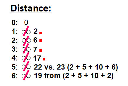
We mark the node with the shortest (currently known) distance equally visited. In this case, node six.

And we cross it off from the listing of unvisited nodes:

Now nosotros have this path (marked in red):

Just one node has non been visited yet, node 5. Let's see how nosotros tin include information technology in the path.

At that place are three unlike paths that nosotros tin can have to achieve node 5 from the nodes that have been added to the path:

• Pick one: 0 -> 1 -> 3 -> v with a distance of 22 (2 + 5 + 15).
• Choice 2: 0 -> 1 -> 3 -> 4 -> 5 with a altitude of 23 (2 + 5 + x + 6).
• Option 3: 0 -> 1 -> three -> four -> 6 -> 5 with a distance of 25 (2 + 5 + 10 + 2 + 6).

We select the shortest path: 0 -> 1 -> iii -> v with a distance of 22.

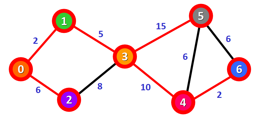
We mark the node as visited and cross it off from the list of unvisited nodes:

And voilà! We have the last result with the shortest path from node 0 to each node in the graph.

In the diagram, the red lines mark the edges that belong to the shortest path. You demand to follow these edges to follow the shortest path to accomplish a given node in the graph starting from node 0.

For example, if y'all desire to achieve node 6 starting from node 0, you just need to follow the cherry edges and you will be following the shortest path 0 -> one -> 3 -> 4 - > 6 automatically.

🔸 In Summary

• Graphs are used to model connections between objects, people, or entities. They have two main elements: nodes and edges. Nodes represent objects and edges represent the connections between these objects.
• Dijkstra's Algorithm finds the shortest path betwixt a given node (which is called the "source node") and all other nodes in a graph.
• This algorithm uses the weights of the edges to find the path that minimizes the full altitude (weight) between the source node and all other nodes.

I actually promise you liked my article and found it helpful. Now you lot know how Dijkstra'south Algorithm works behind the scenes. Follow me on Twitter @EstefaniaCassN and check out my online courses.

---

---

Learn to code for free. freeCodeCamp'southward open source curriculum has helped more than than xl,000 people go jobs as developers. Get started

Source: https://www.freecodecamp.org/news/dijkstras-shortest-path-algorithm-visual-introduction/

Posted by: leehaturat.blogspot.com

Share this post